22. Januar 2013
Inspecting Algorithms with Graphs
 Graphs and algorithms are tightly connected. One surprisingly simple way to inspect algorithms graphically is to let the algorithms plot graphs during their execution using GML (Graph Modeling Language). The produced graphs can be formatted with graph editing software.
The computational complexity of recursive algorithms is often analyzed by counting the number of nodes in the recursion tree (see [1]). But sometimes I like to just see the recursion tree and get an intuitive feeling about what the tree looks like.
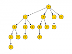
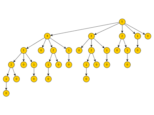
One example is the plain recursive implementation of the rod-cutting algorithm. Note that there is a much more efficient solution to the rod-cutting problem using dynamic programming (see [1]). In order to visualize the exponential complexity of the plain recursive algorithm (and hence why it is bad), we can decorate the algorithm with some plotting statements. A quite concise and simple plotting format is GML (Graph Modelling Language). I prefer to just encode the graph in GML, and let a graph editing software such as yED do the layout.
#include <algorithm>
#include <iostream>

int cut_rod(int *p, int n, int &id) {
    static int nid = 0;
    std::cout << "node" << std::endl
              << "[" << std::endl
              << "id " << nid << std::endl
              << "label " << n << std::endl
              << "]" << std::endl;
    id = nid;
    nid++;
    if (n == 0) {
        return 0;
    } else {
        int q = -1;
        for (int i = 1; i <= n; i++) {
            int cid;
            q = std::max(q, p[i-1] + cut_rod(p, n - i, cid));
            std::cout << "edge" << std::endl
                      << "[" << std::endl
                      << "source " << id << std::endl
                      << "target " << cid << std::endl
                      << "]" << std::endl;
        }
        return q;
    }
}

int main() {
    const int n = 4;
    int p[n];
    std::fill(p, p + n, 0);
    int id;
    std::cout << "graph" << std::endl
              << "[" << std::endl
              << "hierarchic 1" << std::endl
              << "directed 1" << std::endl;
    cut_rod(p, n, id);
    std::cout << "]" << std::endl;
    return 0;
}
The algorithm follows the pseudo-code given in [1] (named CUT-ROD), the example prices for the different rod lengths are all initialized to zero, but here the focus is only on the recursion tree. The produced graph, layouted with yED, looks like this (for n = 5):
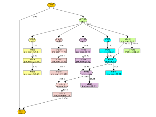
Another example is a parallelized algorithm for computing the line-of-sight using a parallel scan from the Intel Threading Building Blocks (Intel TBB). Here, we are facing an additional difficulty: it is up to Intel TBB to distribute parts of the problem onto different threads. Also the decision about the order of splitting input data and joining partial results is up to Intel TBB, Hence, it is not so easy to reason about what execution paths the parallelized algorithm might take. Here is an automatically generated plot for the execution of a parallel scan (German speakers can read more about the example in context):
Altogether, this is quite a comfortable way to inspect algorithms graphically.
References
[1] T. H. Cormen, C. E. Leiserson, R. L. Rivest, and C. Stein, Introduction to Algorithms, 3rd ed. MIT Press, 2009.