28. Mai 2018
Analysing Strava activities using Colab, Pandas & Matplotlib (Part 1)
 How do you analyse Strava activities—such as runs or bike rides—with Colab, Python, Pandas, and Matplotlib? In this post, I am demonstrating how to get started, and will give you a taster of what is possible with this state-of-the-art technology for data analysis.
I am both curious and skeptical. I love running. And I also happen to like statistics. You won’t be suprised if I tell you now that I find the following questions interesting:
- Do I run longer distances on the weekend than during the week?
- Do I run faster on the weekend than during the week?
- How many days do I rest compared to days I run?
- How many kilometers did I cover during run-commutes?
- Which month of the year do I run the fastest?
- Which month of the year do I run the longest distance?
- Which quarter of the year do I run the fastest?
- Which quarter of the year do I run the longest distance?
- How has the average distance per run changed over the years?
- How has the average time per run changed over the years?
- How has my average speed per run changed over the years?
- How much distance did I run in races and how much during training?
- and so on and so on…
If you’re bored by now, that’s okay. Maybe you better stop reading here. However, should you be curious how to answer these questions by analysing sports activities with Colab, Python, Pandas, and Matplotlib, continue reading.
If you have not heard of Colab, Pandas, Matplotlib before—that’s okay! You should still be able to get a picture of what these are capable of.
- Strava: a mobile application that allows you to track athletic activities. See www.strava.com.
- Colab: a Python notebook highly suited for data analysis using a “literal-programming” style. See colab.research.google.com.
- Pandas: open-source library providing data structures and data analysis tools for Python. See pandas.pydata.org.
- Matplotlib: a 2D plotting library for Python. See matplotlib.org.
Strava provides various tables and visualizations on its website. But I find that Strava rarely happens to visualize the data in a way that answers my questions. What to do?
Outline of steps
The solution I describe here is to export all the activities recorded with Strava to a comma-separated values file (CSV)—runs, bike trips, hiking trips, and ice-skating trips. Then load the activities into Pandas data frames, and use these data frames to analyse and plot the activities.
- request all activities from Strava (instructions) as a zip archive
- import activities.csv from the zip archive into Google Sheets (instructions)
- create a new Colab (instructions)
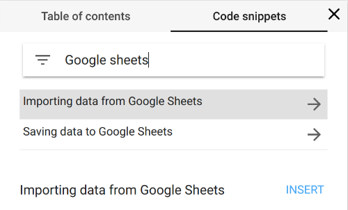
- import data from Google Sheets into Colab (use the snippet “Importing data from Google Sheets”)
- use Pandas to transform and process the activities
- use Matplotlib for creating visualizations
I am not going to provide a detailed walkthrough here—you can look at the Colab.
Download Colab notebook
File: Analysing_Strava_activities_using_Colab,_Pandas_and_Matplotlib_(Part_1).ipynb [6.45 kB]
Category:
Download: 1085
You can open this Colab notebook using Go to File>Upload Notebook… in Colab.
Getting started
In the following, I will explain some key steps in how to get started with analysing your Strava activities.
It is easy to load data from CSV files, Microsoft Excel spreadsheets, or Google Sheets into a Pandas data frame.
As the very first step, we can take out all your data on Strava ( (instructions). In the zip archive, we will find an activities.csv file containing a list of all your activities. We can then upload this CSV file to Google Drive and convert it into a Google Sheet. Then we can insert a snippet into a Colab document, which loads the Google Sheet into a Pandas data frame.
Alternatively, you could probably also adjust the sharing settings of the CSV file in Google Drive to make the file readable by anyone with the link, and then use the pandas.read_csv function to import the data from the CSV file. Whatever works best for you…
Preparing the data
Assuming that we have loaded a Google Sheet into the variable worksheet, we can then create a Pandas data frame.
import pandas as pd
rows = worksheet.get_all_values()
activities_raw = pd.DataFrame.from_records(rows[1:], columns=rows[0]);
The data frame activities_raw holds the unprocessed data from the spreadsheet. Now follows a typical step, and that is transforming the data into a shape that makes it easy to do further data analysis. Let us copy the raw data before modifying it just so that we can avoid reloading the data.
#@title Index activities, convert data types, convert units
activities = activities_raw.copy()
Not all of the columns in the exported Strava activities are relevant; we can easily retain only a few columns. In this case, the time at which the activity started, the type of the activity (“Run”, “Hike”, “Ride”, “IceSkate”), the distance, the duration, whether the activity was a commute to work, and the name of the activity.
# Project
activities = activities[[
    'date', 'type',
    'distance', 'elapsed_time',
    'commute', 'name'
]]
Let us explicitly convert the columns to the desired data types. This drastically simplifies further processing as we can now rely on Pandas doing the right thing when e.g. summing the values in a column. In this case, let us choose date and type as the (multi-)index.
# Set data types
activities['distance'] = activities['distance'].astype(float)
activities['elapsed_time'] = activities['elapsed_time'].astype(float)
activities['commute'] = activities['commute'].apply(lambda x: 1 if x == 'TRUE' else 0)
Let us now convert the distance from meters to kilometers, and the elapsed time from seconds to minutes—this makes sense for me because I find minutes per kilometer intuitive as a measure of pace.
# Convert units
activities['distance'] = activities['distance'] / 1000
activities['elapsed_time'] = activities['elapsed_time'] / 60
Finally, and this is a crucial step in Pandas, let us define the index for the dataframe such that we can easily address each activity by date and type. This makes it very easy to group activities by date and/or by type. Then we can show statistics for running only, or compare activity types.
If you are unfamiliar with Pandas data frames, the index of a data frame is somewhat similar to the primary key of a table in a relational database—although the index of a data frame does not have to be unique.
# Index
activities['date'] = pd.to_datetime(activities_raw['date'])
activities.set_index(['date', 'type'], inplace=True)
Answering basic questions
Let’s look at some of the data.
print(
    activities[['distance', 'elapsed_time']]
      .sample(5)
      .sort_index()
      .to_string(formatters={
          'distance': '{:.0f}km'.format,
          'elapsed_time':' {:.0f}min'.format,
      }))
This shows five randomly selected rows from the data frame.
                        distance elapsed_time
date                type
2015-02-01 10:06:52 Hike     25km       419min
2015-04-06 10:58:24 Run      11km        84min
2016-08-31 08:01:32 Ride      5km        22min
2016-10-05 18:02:36 Ride      6km        29min
2017-10-07 08:01:57 Run      78km      1068min
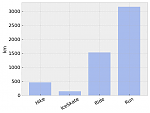
Getting the data into an appropriate format is crucial for further analysis. We are now in a good shape. Let’s have a look for which type of activity I have the most recordings, and in which activity I have covered the most distance:
print(
    activities['distance']
      .groupby(level='type')
      .agg(['count', 'sum'])
      .sort_values(by='count', ascending=False)
      .to_string(formatters={'sum':' {:.0f}km'.format}))
This prints:
         count     sum
type
Run         255  3153km
Ride        100  1526km
Hike         17   465km
IceSkate      3   146km
Let us find out over which time period these activities were recorded:
first_date = activities.index.levels[0].min()
last_date = activities.index.levels[0].max()
print('Activities recorded from %s to %s, total of %d days.' % (
    first_date.strftime('%Y-%m-%d'),
    last_date.strftime('%Y-%m-%d'),
    (last_date - first_date).days))
This prints:
Activities recorded from 2014-06-23 to 2018-05-26, total of 1433 days.
So almost four years of data! We need to be careful, though. The data shows only the activities that were recorded on Strava. I know that I have not always recorded bike rides, hikes, and ice-skating trips. In contrast, I have been diligently recording almost all of my runs over the past years; for running, the least amount of data is missing.
What is next
You might rightly ask. So why use Colab, Python, Pandas, Matplotlib to perform this basic data analysis? We could as well just have used Google Sheets or Microsoft Excel to convert between units, compute sums, create pivot tables and so on; this most likely would have been far easier to do. I am not going to compare between the different tools for data analysis. In the next articles, I will look at the unanswered “research” questions stated above, and to answer these, we need to perform more complex analysis of the data—here we will reap the benefits of our investment to get the activities into the right format. This is where Colab, Pandas, and Matplotlib will shine. Stay tuned.
Read the next article in this series