6. April 2019
Applying Machine Learning to Strava activities using BigQuery ML
 Today, I’ll demo how to train a logistic regression model in BigQuery ML. That is Machine Learning models written in SQL, and executed in BigQuery.
All of what I am writing here is my personal opinion, and not written in any affiliation with Google.
Have you ever wondered whether you can do Machine Learning with SQL only? I had not, but when I heard of BigQuery ML, I got curious,and gave it a shot. You can think of BigQuery as managed storage and a query engine. You can think of BigQuery ML as managed storage + query engine + basic machine learning.
To play around, I chose a dataset I am very familiar with: a list of sports activities exported from Strava. This was a similar dataset (just from a different date) than the dataset I used in my previous articles on Colab, Pandas & Matplotlib:
- Analysing Strava activities using Colab, Pandas & Matplotlib: Part 1
- Analysing Strava activities using Colab, Pandas & Matplotlib Part 2
- Analysing Strava activities using Colab, Pandas & Matplotlib Part 3
- Analysing Strava activities using Colab, Pandas & Matplotlib Part 4
Each activity (row) in the table of activities has the following fields (among others):
- id (INTEGER)
- date (TIMESTAMP)
- name (STRING)
- type (STRING)
- elapsed_time (INTEGER)
- distance (FLOAT)
- commute (BOOLEAN)
Let us predict whether a given activity recorded on Strava was a commute or not. I will skip over the usual steps of exploring the data, and cleaning the data because I know the data very well. So let’s go ahead and split the data deterministically into a training set (around 80%) and test set (around 20%) by hashing the identifier, which remains stable when running the queries again.
create or replace table `strava.training_set` as
select
  *,
  (extract(dayofweek from date) = 1
    or extract(dayofweek from date) = 7) as weekend
from `strava.activities`
where
  mod(abs(id), 10) < 8
  and commute is not null
Note here that we discard entries from the training set where no value was recorded for the commute label.
create or replace table `strava.test_set` as
select
  *,
  (extract(dayofweek from date) = 1
    or extract(dayofweek from date) = 7) as weekend
from `strava.activities`
where
  mod(abs(id), 10) >= 8
That’s done. Now, I have one tables of activities for use as a training set (381 rows), and one table of activities for use as a test set (86 rows). I will hold the test set aside until the very end when I have finished training the models.
Once you remember the syntax, training a logistic regression model for classification is pretty straight-forward. Let’s start with a simple model which tries to predict whether an activity was a commute based on the distance. I know that the distance is probably a good predictor because commutes tend to have the same distance as opposed e.g. to runs on the weekend.
create or replace model `strava.commute_distance`
options (
  model_type='logistic_reg',
  input_label_cols=['commute']
) as
select
  distance,
  commute
from `strava.training_set`
Let’s also take elapsed time into account.
create or replace model `strava.commute_distance_elapsed_time`
options (
  model_type='logistic_reg',
  input_label_cols=['commute']
) as
select
  distance,
  elapsed_time,
  commute
from `strava.training_set`
It’s quite easy to create a bunch of models, by copy-pasting the SQL query and then adding another feature. Let’s also add a model which takes the type of the activity into consideration. After all, I rarely use ice skates to commute to the office (although I wish I could!). Note how even categorical data works as features without additional prep.
create or replace model `strava.commute_distance_elapsed_time_type`
options (
  model_type='logistic_reg',
  input_label_cols=['commute']
) as
select
  distance,
  elapsed_time,
  type,
  commute
from `strava.training_set`
Finally, I rarely commute to work on weekends, so let’s add that feature as well.
create or replace model `strava.commute_distance_elapsed_time_type_weekend`
options (
  model_type='logistic_reg',
  input_label_cols=['commute']
) as
select
  distance,
  elapsed_time,
  type,
  weekend,
  commute
from `strava.training_set`
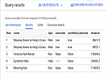
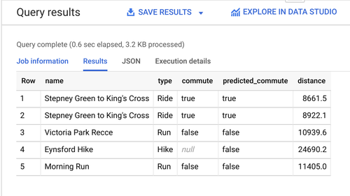
Now I have the models trained, let’s take the simplest one (which only considers distance), and predict a few labels.
select
  name,
  type,
  commute,
  predicted_commute,
  distance
from
  ml.predict(
    model `strava.commute_distance`,
    (select * from `strava.test_set`))
 order by rand()
 limit 5
Okay, but how good is the model actually? How good are the other models? BigQuery ML makes this easy, for it also supports model evaluation. And here is how to do that, for the first model:
select * from
  ml.evaluate(
    model `strava.commute_distance`,
    (select * from `strava.test_set`));
For the second model:
select * from
  ml.evaluate(
    model `strava.commute_distance_elapsed_time`,
    (select * from `strava.test_set`));
For the third model:
select * from
  ml.evaluate(
    model `strava.commute_distance_elapsed_time_type`,
    (select * from `strava.test_set`));
For the fourth model:
select * from
  ml.evaluate(
    model `strava.commute_distance_elapsed_time_type_weekend`,
    (select * from `strava.test_set`));
Putting the results into a table, here are the results of the four models evaluated on the test set. If you look at the ROC AUC, it gets progressively better the more features I added. Of course, as I said, I know the dataset very well, so the choice of features was no accident.
| model | 1 | 2 | 3 | 4 |
| precision | 0.83 | 0.81 | 0.84 | 0.91 |
| recall | 1.0 | 1.0 | 1.0 | 1.0 |
| accuracy | 0.87 | 0.86 | 0.88 | 0.94 |
| f1_score | 0.90 | 0.90 | 0.91 | 0.95 |
| log_loss | 0.49 | 0.45 | 0.46 | 0.23 |
| roc_auc | 0.81 | 0.82 | 0.85 | 0.95 |
And that’s Machine Learning using BigQuery ML.